<?xml version="1.0" encoding="utf-8"?>
<feed xmlns="http://www.w3.org/2005/Atom">
  <title>databait</title>
  
  <link href="/atom.xml" rel="self"/>
  
  <link href="https://databait.github.io/"/>
  <updated>2016-12-12T14:27:27.776Z</updated>
  <id>https://databait.github.io/</id>
  
  <author>
    <name>databait@gmail.com</name>
    
  </author>
  
  <generator uri="http://hexo.io/">Hexo</generator>
  
  <entry>
    <title>The Kelly Criterion in Applied Portfolio Selection - Part 2</title>
    <link href="https://databait.github.io/2016/12/12/The-Kelly-Criterion-in-Applied-Portfolio-Selection-Part-2/"/>
    <id>https://databait.github.io/2016/12/12/The-Kelly-Criterion-in-Applied-Portfolio-Selection-Part-2/</id>
    <published>2016-12-12T12:34:14.000Z</published>
    <updated>2016-12-12T14:27:27.776Z</updated>
    
    <content type="html"><![CDATA[<h3 id="Previous-blog-post-on-the-Kelly-Criterion"><a href="#Previous-blog-post-on-the-Kelly-Criterion" class="headerlink" title="Previous blog post on the Kelly Criterion"></a>Previous blog post on the Kelly Criterion</h3><p>As pointed out in a <a href="/2016/12/10/The-Kelly-Criterion-in-Applied-Portfolio-Selection/">previous blog post</a>, the Kelly Criterion is an interesting option to decide on position sizing in portfolio selection. While the previous post looked at single stocks, I will today show how to optimize position sizes for a portfolio with multiple stocks.</p>
<h3 id="The-core-function"><a href="#The-core-function" class="headerlink" title="The core function"></a>The core function</h3><p>At the core of my portfolio optimization is this function:</p>
<figure class="highlight r"><table><tr><td class="gutter"><pre><div class="line">1</div><div class="line">2</div><div class="line">3</div><div class="line">4</div><div class="line">5</div><div class="line">6</div><div class="line">7</div><div class="line">8</div><div class="line">9</div><div class="line">10</div><div class="line">11</div><div class="line">12</div><div class="line">13</div></pre></td><td class="code"><pre><div class="line">opt_portfolio &lt;-<span class="keyword">function</span>(shares, dpf, maxshare) &#123;</div><div class="line">  </div><div class="line">  <span class="comment"># calculate portfolios return vector</span></div><div class="line">  exp_returns &lt;- dpf%*%shares</div><div class="line">  </div><div class="line">  obj = -sum(log(<span class="number">1</span>+exp_returns))</div><div class="line">  weight.penalty = <span class="number">1000</span>*(<span class="number">1</span>-sum(shares))^<span class="number">2</span></div><div class="line">  </div><div class="line">  <span class="comment"># max share penalty:</span></div><div class="line">  maxpen &lt;- sum(shares[shares&gt;maxshare])*<span class="number">1000</span></div><div class="line"></div><div class="line">  <span class="keyword">return</span>(obj + weight.penalty + maxpen)</div><div class="line">&#125;</div></pre></td></tr></table></figure>
<p>The function has three parameters. <code>shares</code> is the vector of shares (position size for each stock) that is going to be estimated by optimization. <code>dpf</code> is a matrix where each stock is a column and each line contains the daily stock price movements like e.g.: <code>diff(stock)/lag(stock)</code>. The <code>maxshare</code> option can be used to restrict the position size of a single stock to a maximum. </p>
<p><code>exp_returns &lt;- dpf%*%shares</code> calculates the daily (or weekly) portfolio returns. <code>obj</code> is the Kelly Criterion. The higher the volatility, the larger values <code>obj</code> will take. We are going to minimize the function so low values, i.e. low volatility is preferred. The next line is a trick to restrict the optimizer to values that sum to 1 (100%). If the sum of all position sizes is 1, <code>weight.penalty</code> is 0 (the minimum possible value). Would the sum deviate from 1, the <code>weight.penalty</code> would quickly increase. The second penalty term is similar. If a position is sized above the maximum allowed share, the penalty scores. Finally the function returns a value which the optimizer will try to minimize.</p>
<h3 id="The-wrapper-function"><a href="#The-wrapper-function" class="headerlink" title="The wrapper function"></a>The wrapper function</h3><p>Now to feed stock data into this function I wrote a wrapper function that prepares the matrix of returns and calls <code>optim()</code>.</p>
<figure class="highlight r"><table><tr><td class="gutter"><pre><div class="line">1</div><div class="line">2</div><div class="line">3</div><div class="line">4</div><div class="line">5</div><div class="line">6</div><div class="line">7</div><div class="line">8</div><div class="line">9</div><div class="line">10</div><div class="line">11</div><div class="line">12</div><div class="line">13</div><div class="line">14</div><div class="line">15</div><div class="line">16</div><div class="line">17</div><div class="line">18</div><div class="line">19</div><div class="line">20</div><div class="line">21</div><div class="line">22</div><div class="line">23</div><div class="line">24</div><div class="line">25</div><div class="line">26</div><div class="line">27</div><div class="line">28</div><div class="line">29</div><div class="line">30</div><div class="line">31</div><div class="line">32</div><div class="line">33</div><div class="line">34</div><div class="line">35</div><div class="line">36</div><div class="line">37</div><div class="line">38</div><div class="line">39</div><div class="line">40</div><div class="line">41</div><div class="line">42</div><div class="line">43</div><div class="line">44</div><div class="line">45</div><div class="line">46</div><div class="line">47</div><div class="line">48</div><div class="line">49</div></pre></td><td class="code"><pre><div class="line"><span class="keyword">library</span>(quantmod)</div><div class="line"><span class="keyword">library</span>(dplyr)</div><div class="line"></div><div class="line">opt_portfolio_wrapper &lt;- <span class="keyword">function</span>(stocks,r=rep(<span class="number">0.03</span>,length(stocks)),maxshare=<span class="number">1</span>,daily=<span class="literal">FALSE</span>,short=<span class="literal">FALSE</span>) &#123;</div><div class="line">  </div><div class="line">  <span class="comment"># test which stocks are already in workspace, else download data</span></div><div class="line">  <span class="keyword">for</span>(stock <span class="keyword">in</span> stocks) &#123;</div><div class="line">    <span class="keyword">if</span>(!exists(stock)) getSymbols(stock,from=<span class="string">"1970-01-01"</span>,env=parent.frame(<span class="number">2</span>))</div><div class="line">  &#125;</div><div class="line">  </div><div class="line">  <span class="comment"># transform return vector from yearly to daily or weekly</span></div><div class="line">  <span class="keyword">if</span>(daily==<span class="literal">TRUE</span>) &#123;</div><div class="line">    r &lt;- (<span class="number">1</span>+r)^(<span class="number">1</span>/<span class="number">250</span>)-<span class="number">1</span></div><div class="line">  &#125; <span class="keyword">else</span> &#123;</div><div class="line">    r &lt;- (<span class="number">1</span>+r)^(<span class="number">1</span>/<span class="number">52</span>)-<span class="number">1</span></div><div class="line">  &#125;</div><div class="line">  </div><div class="line">  portfolio &lt;- <span class="literal">NULL</span></div><div class="line">  <span class="keyword">for</span>(stock <span class="keyword">in</span> stocks) &#123;</div><div class="line">    <span class="keyword">if</span>(daily) assign(stock,get(stock)[,<span class="number">6</span>])</div><div class="line">    <span class="keyword">if</span>(!daily) assign(stock,to.weekly(get(stock))[,<span class="number">6</span>])</div><div class="line">  &#125;</div><div class="line"></div><div class="line">  <span class="comment"># merge all stocks together</span></div><div class="line">  portfolio &lt;- Reduce(<span class="keyword">function</span>(<span class="keyword">...</span>) merge(<span class="keyword">...</span>, all=<span class="literal">TRUE</span>), mget(stocks))</div><div class="line">  </div><div class="line">  <span class="comment"># build returns by diff()/lag()</span></div><div class="line">  d.portfolio &lt;- data.frame(na.omit(diff(portfolio)/stats::lag(portfolio)))</div><div class="line">  </div><div class="line">  <span class="comment"># center around the mean to eliminate past performance as an information for portfolio selection</span></div><div class="line">  d.portfolio.future &lt;- scale(d.portfolio, scale=<span class="literal">F</span>)</div><div class="line">  </div><div class="line">  <span class="comment"># add the (personally) expected return for each stock</span></div><div class="line">  <span class="keyword">for</span>(i <span class="keyword">in</span> <span class="number">1</span>:ncol(d.portfolio.future)) &#123;</div><div class="line">    d.portfolio.future[,i] &lt;- d.portfolio.future[,i] + r[i]</div><div class="line">  &#125;</div><div class="line">  </div><div class="line">  <span class="comment"># define lower und upper bounds for the parameters. 0 to 1 or -1 to 1 if short positions are allowed</span></div><div class="line">  lower &lt;- rep(ifelse(short==<span class="literal">TRUE</span>,-<span class="number">1</span>,<span class="number">0</span>),length(stocks))</div><div class="line">  upper &lt;- rep(<span class="number">1</span>,length(stocks))</div><div class="line">  </div><div class="line">  <span class="comment"># starting values for optimizer</span></div><div class="line">  start &lt;- rep(<span class="number">1</span>/length(stocks),length(stocks))</div><div class="line">  </div><div class="line">  res &lt;- optim(start, opt_portfolio, dpf=d.portfolio.future, maxshare=maxshare, method=<span class="string">"Nelder-Mead"</span>)</div><div class="line">  </div><div class="line">  Portfolio &lt;- data.frame(<span class="string">"Share"</span>=res$par,<span class="string">"Stock"</span>=stocks) %&gt;% arrange(desc(Share))</div><div class="line">  <span class="keyword">return</span>(Portfolio)</div><div class="line">&#125;</div></pre></td></tr></table></figure>
<p>Most of the function is commented between the lines. I introduced two options: <code>daily</code> and <code>short</code>. The default values are, that short positions are not allowed and the returns are calculated on a weekly, not daily basis. One thing thats important for me is, that I dont use the stock returns as they are but I center them around the mean return that I expect. If I would not do this, the algorithm would always pick the historically best performing stock(s). However past performance is not a good predictor of future performance and one has to do his homework and build own (and realistic) expectations.</p>
<h3 id="Testing"><a href="#Testing" class="headerlink" title="Testing"></a>Testing</h3><p>To test the function I select some random stocks (not a recommendation to trade these stocks).</p>
<figure class="highlight r"><table><tr><td class="gutter"><pre><div class="line">1</div><div class="line">2</div><div class="line">3</div><div class="line">4</div><div class="line">5</div><div class="line">6</div><div class="line">7</div><div class="line">8</div><div class="line">9</div></pre></td><td class="code"><pre><div class="line">rstocks &lt;- c(<span class="string">"AAPL"</span>,<span class="string">"GOOG"</span>,<span class="string">"AMZN"</span>,<span class="string">"GIS"</span>)</div><div class="line"></div><div class="line">opt_portfolio_wrapper(rstocks)</div><div class="line"></div><div class="line"><span class="comment">#        Share Stock</span></div><div class="line"><span class="comment"># 1 0.80851815   GIS</span></div><div class="line"><span class="comment"># 2 0.09979312  AAPL</span></div><div class="line"><span class="comment"># 3 0.06343397  GOOG</span></div><div class="line"><span class="comment"># 4 0.02829082  AMZN</span></div></pre></td></tr></table></figure>
<p>This tells the following story: Assuming all stocks have the same expected yearly return of 3%, the long term growth rate of wealth (Kelly Criterion) is achieved by investing in the stock with a lowest volatility (here GIS). At the same time this is a hint, that the assumption that all returns are to be expected as equal is too strong. One could now play with the function to find out how high the expected return of a risky stock has to be, to be included into an existing portfolio. </p>
<h3 id="Summary"><a href="#Summary" class="headerlink" title="Summary"></a>Summary</h3><p>I personally use this tool as a rough orientation, how stocks from my watchlist would contribute to the risk-return-profile of my portfolio. I usually use the <code>maxshare</code> option and rather “flat” and moderate return expectations, because the Kelly Criterion highly favors stocks with better return expectations. E.g. if I add 1% additional expected return for GOOG, the numbers change drastically:</p>
<figure class="highlight r"><table><tr><td class="gutter"><pre><div class="line">1</div><div class="line">2</div><div class="line">3</div><div class="line">4</div><div class="line">5</div><div class="line">6</div><div class="line">7</div></pre></td><td class="code"><pre><div class="line">opt_portfolio_wrapper(rstocks, r=c(<span class="number">0.03</span>,<span class="number">0.04</span>,<span class="number">0.03</span>,<span class="number">0.03</span>))</div><div class="line"></div><div class="line"><span class="comment">#          Share Stock</span></div><div class="line"><span class="comment"># 1  0.749115293   GIS</span></div><div class="line"><span class="comment"># 2  0.200639803  GOOG</span></div><div class="line"><span class="comment"># 3  0.051410711  AAPL</span></div><div class="line"><span class="comment"># 4 -0.001125542  AMZN</span></div></pre></td></tr></table></figure>
<p>If find the tool to be useful because it keeps me from overbetting on very volatile stocks and gives hints, if and when risky stocks are worth to bet on. </p>
<h3 id="Other"><a href="#Other" class="headerlink" title="Other"></a>Other</h3><p>There are a few additional points worth mentioning:</p>
<ul>
<li>while <code>opt_portfolio_wrapper()</code> gives the shares to achieve the Kelly-optimal portfolio selection, it does not tell, how much one should bet on the whole portfolio. Approximately this be calculated by dividing the expected portfolio return by the annualized variance. One could also adapt the <code>kelly()</code> function from the <a href="/2016/12/10/The-Kelly-Criterion-in-Applied-Portfolio-Selection/">previous blog post</a> to get a number that incorporates the fact, that the return distribution is fat-tailed and non-normal.</li>
<li>I excluded some of the options that my function originally had for the sake of readability. Options that I found interesting are:<ul><li>transaction costs<br></li><li>“fixed shares” (e.g. my pension account is invested in index funds and bonds. When picking stocks, I might want to incorporate the fact, that I am already exposed to these securities)<br></li><li>a <code>from</code> option for <code>getSymbols()</code> if the historic returns should be restricted to a certain range</li></ul></li>
</ul>
]]></content>
    
    <summary type="html">
    
      &lt;h3 id=&quot;Previous-blog-post-on-the-Kelly-Criterion&quot;&gt;&lt;a href=&quot;#Previous-blog-post-on-the-Kelly-Criterion&quot; class=&quot;headerlink&quot; title=&quot;Previous b
    
    </summary>
    
    
      <category term="R" scheme="https://databait.github.io/tags/R/"/>
    
      <category term="Finance" scheme="https://databait.github.io/tags/Finance/"/>
    
  </entry>
  
  <entry>
    <title>The Kelly Criterion in Applied Portfolio Selection</title>
    <link href="https://databait.github.io/2016/12/10/The-Kelly-Criterion-in-Applied-Portfolio-Selection/"/>
    <id>https://databait.github.io/2016/12/10/The-Kelly-Criterion-in-Applied-Portfolio-Selection/</id>
    <published>2016-12-10T22:52:39.000Z</published>
    <updated>2016-12-11T19:23:10.004Z</updated>
    
    <content type="html"><![CDATA[<h3 id="The-Kelly-Criterion"><a href="#The-Kelly-Criterion" class="headerlink" title="The Kelly Criterion"></a>The Kelly Criterion</h3><p><a href="http://www.herrold.com/brokerage/kelly.pdf" target="_blank" rel="external">Derived by John L. Kelly (1956)</a> the criterion recommends a certain fraction of a bankroll to be put on a bet with positive expectations. Kelly showed that $$\frac{p \cdot (b+1) - 1}{b}$$ optimizes the growth rate of wealth if the game to bet on is repeated for many times, where <i>p</i> is the probability to win the bet and <i>b</i> is the net odds, i.e. what you would get back in excess of amount wagered. For example if you are offered to get your wager tripled for a correct coin flip guess, the Kelly criterion would advice you to bet $$\frac{0.5 * (2+1) - 1}{2} = 0.25$$.</p>
<p>While the concept is popular in the betting universe and sometimes in options trading, it seems not to be a common concept in portfolio selection. However, the concept is rather easy to transfer into portfolio selection as all it does is optimizing the long term growth rate. What we would like to find is the fraction that optimizes the following function:</p>
<figure class="highlight r"><table><tr><td class="gutter"><pre><div class="line">1</div><div class="line">2</div><div class="line">3</div></pre></td><td class="code"><pre><div class="line">sum_logx &lt;- <span class="keyword">function</span>(f,x) &#123;</div><div class="line">  -sum(log(<span class="number">1</span>+f*x))</div><div class="line">&#125;</div></pre></td></tr></table></figure>
<p><code>x</code> is a vector of expected future returns of a stock (which we yet have to conceptualize) and <code>f</code> is the fraction to be calculated. First of all we need to make assumptions about our expected return. As an example lets assume we expect 3% annualized return for a stock (e.g. because that is approximately in line with economic growth expectations). Second we need to make assumptions about the underlying risk/volatility. I derive the risk from the history of returns. At this point I often get criticized from the value investors camp because it has a flavor of efficient market hypothesis, beta, Black-Scholes, capital asset pricing model (CAPM), LTCM crash, etc. </p>
<p>Here is my few arguments why basing future risk on past risk seems legit to me:</p>
<ol>
<li>Past and present risk (absolute values of daily returns) are highly correlated</li>
<li>The risky stocks from yesterday usually are the risky stocks of tomorrow</li>
<li>NOT using historical information of volatility at all cannot be better</li>
<li>If you believe that volatility is not the whole picture of risk, there are ways to incorporate additional measures of risk (as we will see later)</li>
</ol>
<p>By looking at the <code>sum_logx</code> function, one can see that the Kelly criterion relaxes the strong assumptions that are implicit in the CAPM (normally distributed independent returns, constant correlation between assets) because it recognizes each data point “as is”, and NOT averaging out outliers by calculating a standard deviation. Therefore, more realistically, the Kelly criterion is capable of covering a huge part of the fat tails of the return distribution. </p>
<h3 id="An-example"><a href="#An-example" class="headerlink" title="An example"></a>An example</h3><p>I use the Amazon stock as a mere example. This is not a recommendation to trade the stock.</p>
<figure class="highlight r"><table><tr><td class="gutter"><pre><div class="line">1</div><div class="line">2</div><div class="line">3</div><div class="line">4</div></pre></td><td class="code"><pre><div class="line"><span class="keyword">library</span>(quantmod)</div><div class="line"></div><div class="line">stock &lt;- <span class="string">"AMZN"</span> <span class="comment"># Stock of Amazon</span></div><div class="line">getSymbols(stock, from=<span class="string">"2007-01-01"</span>)</div></pre></td></tr></table></figure>
<p>Using the very early days of Amazon is probably not representative for the future risk, as Amazon matured. However the time span should ideally include all aspects of economic cycles, so I used about 10 years, including the financial crisis 2008.</p>
<p>Now I calculate weekly and monthly returns based on the adjusted closing price.</p>
<figure class="highlight r"><table><tr><td class="gutter"><pre><div class="line">1</div><div class="line">2</div><div class="line">3</div><div class="line">4</div></pre></td><td class="code"><pre><div class="line">stock.m &lt;- to.monthly(get(stock))[,<span class="number">6</span>]</div><div class="line">stock.w &lt;- to.weekly(get(stock))[,<span class="number">6</span>]</div><div class="line">d.stock.m &lt;- as.numeric(na.omit(diff(stock.m)/lag(stock.m)))</div><div class="line">d.stock.w &lt;- as.numeric(na.omit(diff(stock.w)/lag(stock.w)))</div></pre></td></tr></table></figure>
<p>Now to incorporate my expected return I center the time series around that value. One might argue about the procedure but I find it more plausible than e.g. putting past returns into my models (as some people do) since past returns are not a predictor of future returns. So this is my best guestimate. </p>
<figure class="highlight r"><table><tr><td class="gutter"><pre><div class="line">1</div><div class="line">2</div><div class="line">3</div><div class="line">4</div><div class="line">5</div><div class="line">6</div><div class="line">7</div></pre></td><td class="code"><pre><div class="line">r &lt;- <span class="number">0.03</span> <span class="comment"># annualized return</span></div><div class="line">r.m &lt;- (<span class="number">1</span>+r)^(<span class="number">1</span>/<span class="number">12</span>)-<span class="number">1</span> <span class="comment"># monthly</span></div><div class="line">r.w &lt;- (<span class="number">1</span>+r)^(<span class="number">1</span>/<span class="number">52</span>)-<span class="number">1</span> <span class="comment"># weekly</span></div><div class="line"></div><div class="line"><span class="comment"># now subtract mean of past return and add expected return.</span></div><div class="line">stock.future.m &lt;- d.stock.m - mean(d.stock.m) + r.m</div><div class="line">stock.future.w &lt;- d.stock.w - mean(d.stock.w) + r.w</div></pre></td></tr></table></figure>
<p>With this I basically keep the empiric distribution of returns to represent risk and input my personal expectation. </p>
<p>Then I optimize the function <code>sumlog_x</code> using the defined vectors of expected returns for both, weekly and monthly returns.</p>
<figure class="highlight r"><table><tr><td class="gutter"><pre><div class="line">1</div><div class="line">2</div><div class="line">3</div><div class="line">4</div></pre></td><td class="code"><pre><div class="line">optim(par=<span class="number">0.2</span>,fn=sum_logx,x=stock.future.m)$par <span class="comment"># par being the starting value of the optimizer</span></div><div class="line"><span class="comment"># [1] 0.2282031</span></div><div class="line">optim(par=<span class="number">0.2</span>,fn=sum_logx,x=stock.future.w)$par</div><div class="line"><span class="comment"># [1] 0.2045313</span></div></pre></td></tr></table></figure>
<p>This comes up with numbers around 20% of bankroll. Keep in mind however, that this relies on the assumptions, that the expected return is 3% and the return distribution of the next year is expected to be of the same source as was the return distribution in the last decade. Furthermore it is important, that overbetting does more harm than underbetting. Therefore many people recommend betting “half Kelly” to be rather on the save side that is slightly underperforming than on the risky side, that waits for the big wave to be wiped out.</p>
<p>Now what if I wanted an even more conservative estimate? Lets assume I expect the risk of bankruptcy for the next twelve month to be 0.4% higher than it is reflected by the market. I went for this very simple solution:</p>
<figure class="highlight r"><table><tr><td class="gutter"><pre><div class="line">1</div><div class="line">2</div><div class="line">3</div><div class="line">4</div></pre></td><td class="code"><pre><div class="line">d.stock.m &lt;- c(d.stock.m,rep(-<span class="number">1</span>,<span class="number">10</span>))</div><div class="line">d.stock.w &lt;- c(d.stock.w,rep(-<span class="number">1</span>,<span class="number">10</span>))</div><div class="line">stock.future.m &lt;- d.stock.m - mean(d.stock.m) + r.m</div><div class="line">stock.future.w &lt;- d.stock.w - mean(d.stock.w) + r.w</div></pre></td></tr></table></figure>
<p>For each of the 10 years, I include one (~0.4%) total loss (-1). In my opinion it is always advisable to think about total loss probability because listed stocks are per definition the ones that are not (yet) bankrupt (survivorship bias). The empiric distribution (my approach) has much fatter tails than the normal distribution (conventional approach) but it does not cover the events that did not take place so far. </p>
<figure class="highlight r"><table><tr><td class="gutter"><pre><div class="line">1</div><div class="line">2</div><div class="line">3</div><div class="line">4</div></pre></td><td class="code"><pre><div class="line">optim(par=<span class="number">0.2</span>,fn=sum_logx,x=stock.future.m)$par <span class="comment"># par being the starting value of the optimizer</span></div><div class="line"><span class="comment"># [1] 0.02796875</span></div><div class="line">optim(par=<span class="number">0.2</span>,fn=sum_logx,x=stock.future.w)$par</div><div class="line"><span class="comment"># [1] 0.02576172</span></div></pre></td></tr></table></figure>
<h3 id="Summary"><a href="#Summary" class="headerlink" title="Summary"></a>Summary</h3><p>As can be seen, the Kelly criterion is rather optimistic in general but very sensitive to total losses. I use the procedure as a tool to get a first impression of a stock I am thinking to invest in. However there is more to be looked at, e.g. the diversification benefit of the stock within an existing portfolio. I will cover this topic - how to optimize the Kelly criterion for a portfolio of multiple stocks - in a subsequent post.</p>
<h3 id="Appendix-Kelly-Criterion-as-an-R-function"><a href="#Appendix-Kelly-Criterion-as-an-R-function" class="headerlink" title="Appendix: Kelly Criterion as an R-function"></a>Appendix: Kelly Criterion as an R-function</h3><p>For convenience here is the code of the function I use:</p>
<figure class="highlight r"><table><tr><td class="gutter"><pre><div class="line">1</div><div class="line">2</div><div class="line">3</div><div class="line">4</div><div class="line">5</div><div class="line">6</div><div class="line">7</div><div class="line">8</div><div class="line">9</div><div class="line">10</div><div class="line">11</div><div class="line">12</div><div class="line">13</div><div class="line">14</div><div class="line">15</div><div class="line">16</div><div class="line">17</div><div class="line">18</div><div class="line">19</div><div class="line">20</div><div class="line">21</div><div class="line">22</div><div class="line">23</div><div class="line">24</div><div class="line">25</div><div class="line">26</div><div class="line">27</div><div class="line">28</div><div class="line">29</div></pre></td><td class="code"><pre><div class="line">sum_logx &lt;- <span class="keyword">function</span>(f,x) &#123;</div><div class="line">  -sum(log(<span class="number">1</span>+f*x))</div><div class="line">&#125;</div><div class="line"></div><div class="line"><span class="keyword">library</span>(quantmod)</div><div class="line"></div><div class="line">kelly &lt;- <span class="keyword">function</span>(stock,r=<span class="number">0.03</span>,from=<span class="string">"1970-01-01"</span>,blowups=<span class="number">0</span>,par=<span class="number">0.2</span>) &#123;</div><div class="line">  getSymbols(stock,from=from,env=parent.frame(<span class="number">2</span>))</div><div class="line">  stock.m &lt;- to.monthly(get(stock))[,<span class="number">6</span>]</div><div class="line">  stock.w &lt;- to.weekly(get(stock))[,<span class="number">6</span>]</div><div class="line">  d.stock.m &lt;- as.numeric(na.omit(diff(stock.m)/lag(stock.m)))</div><div class="line">  d.stock.w &lt;- as.numeric(na.omit(diff(stock.w)/lag(stock.w)))</div><div class="line">  r.m &lt;- (<span class="number">1</span>+r)^(<span class="number">1</span>/<span class="number">12</span>)-<span class="number">1</span></div><div class="line">  r.w &lt;- (<span class="number">1</span>+r)^(<span class="number">1</span>/<span class="number">52</span>)-<span class="number">1</span></div><div class="line">  <span class="keyword">if</span>(blowups&gt;<span class="number">0</span>) &#123;</div><div class="line">    d.stock.m &lt;- c(d.stock.m,rep(-<span class="number">1</span>,blowups))</div><div class="line">    d.stock.w &lt;- c(d.stock.w,rep(-<span class="number">1</span>,blowups))</div><div class="line">  &#125;</div><div class="line">  stock.future.m &lt;- d.stock.m-mean(d.stock.m)+r.m </div><div class="line">  stock.future.w &lt;- d.stock.w-mean(d.stock.w)+r.w</div><div class="line">    <span class="keyword">return</span>(list(</div><div class="line">      <span class="string">"Monthly"</span>=optim(par=par,fn=sum_logx,x=stock.future.m)$par,</div><div class="line">      <span class="string">"Weekly"</span>=optim(par=par,fn=sum_logx,x=stock.future.w)$par,</div><div class="line">      <span class="string">"Timeframe"</span>=nrow(get(stock))))</div><div class="line">&#125;</div><div class="line"></div><div class="line"><span class="comment"># use like this:</span></div><div class="line">kelly(<span class="string">"AAPL"</span>)</div><div class="line">kelly(<span class="string">"MSFT"</span>,blowups=<span class="number">2</span>)</div></pre></td></tr></table></figure>
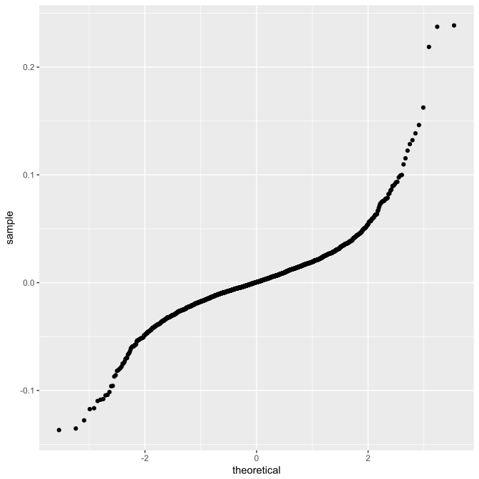
<h3 id="Appendix-Fat-tails"><a href="#Appendix-Fat-tails" class="headerlink" title="Appendix: Fat tails"></a>Appendix: Fat tails</h3><p>As mentioned above, stock returns are not normally distributed, therefore the CAPM compared to advise from the Kelly criterion tends to “overbet”. </p>
<figure class="highlight r"><table><tr><td class="gutter"><pre><div class="line">1</div><div class="line">2</div><div class="line">3</div><div class="line">4</div><div class="line">5</div><div class="line">6</div></pre></td><td class="code"><pre><div class="line"><span class="keyword">library</span>(quantmod)</div><div class="line"><span class="keyword">library</span>(ggplot2)</div><div class="line"></div><div class="line">getSymbols(<span class="string">"AMZN"</span>, from=<span class="string">"2007-01-01"</span>)</div><div class="line">empiric_returns &lt;- na.omit(diff(log(AMZN[,<span class="number">6</span>])))</div><div class="line">ggplot(data.frame(empiric_returns), aes(sample=empiric_returns)) + stat_qq()</div></pre></td></tr></table></figure>
<p><img src="/images/qqplot.svg" alt=""></p>
<p>Plotting the empiric quantiles vs. the theoretical quantiles we see that returns outside of the range of two standard deviations left and right is much more frequent than the normal distribution would suggest. This combined with high leverage was the central reason for the <a href="https://en.wikipedia.org/wiki/Long-Term_Capital_Management#Downturn" target="_blank" rel="external">collapse of LTCM</a>.</p>
]]></content>
    
    <summary type="html">
    
      &lt;h3 id=&quot;The-Kelly-Criterion&quot;&gt;&lt;a href=&quot;#The-Kelly-Criterion&quot; class=&quot;headerlink&quot; title=&quot;The Kelly Criterion&quot;&gt;&lt;/a&gt;The Kelly Criterion&lt;/h3&gt;&lt;p&gt;&lt;a
    
    </summary>
    
    
      <category term="R" scheme="https://databait.github.io/tags/R/"/>
    
      <category term="Finance" scheme="https://databait.github.io/tags/Finance/"/>
    
  </entry>
  
  <entry>
    <title>Webscraping with R using a Raspberry Pi</title>
    <link href="https://databait.github.io/2016/12/08/Webscraping-with-R-using-a-Raspberry-Pi/"/>
    <id>https://databait.github.io/2016/12/08/Webscraping-with-R-using-a-Raspberry-Pi/</id>
    <published>2016-12-08T01:08:08.000Z</published>
    <updated>2016-12-11T13:35:11.423Z</updated>
    
    <content type="html"><![CDATA[<h3 id="Setting-up-the-Raspberry-Pi"><a href="#Setting-up-the-Raspberry-Pi" class="headerlink" title="Setting up the Raspberry Pi"></a>Setting up the Raspberry Pi</h3><p>After the basic setup, i.e.</p>
<ul>
<li>bought a Raspberry Pi Starter Kit</li>
<li>flashed the SD Card with <a href="https://www.raspbian.org/" target="_blank" rel="external">Raspbian</a></li>
<li>ran <code>raspi-config</code></li>
<li>installed R with <code>apt-get install R</code>, which installed R 3.1.1</li>
</ul>
<p>I started to install the R packages usually needed for my cron-job tasks (mostly webscraping). I ran into problems with the <code>rvest</code> package because several packages could not be installed. Maybe there is a more efficient way but I did the following steps:</p>
<h3 id="Install-packages-for-webscraping"><a href="#Install-packages-for-webscraping" class="headerlink" title="Install packages for webscraping"></a>Install packages for webscraping</h3><p>To install xml and related R packages (rvest), I needed the libxml2 on the system although apt-get had it, so I manually installed it:</p>
<figure class="highlight bash"><table><tr><td class="gutter"><pre><div class="line">1</div><div class="line">2</div><div class="line">3</div></pre></td><td class="code"><pre><div class="line">wget ftp://xmlsoft.org/libxml2/libxml2-2.9.2.tar.gz</div><div class="line">tar -xzvf libxml2-2.9.2.tar.gz</div><div class="line"><span class="built_in">cd</span> libxml2-2.9.2/</div></pre></td></tr></table></figure>
<p>I also needed python-dev to make libxml2 compile.</p>
<figure class="highlight bash"><table><tr><td class="gutter"><pre><div class="line">1</div><div class="line">2</div></pre></td><td class="code"><pre><div class="line">sudo apt-get update</div><div class="line">sudo apt-get install python-dev</div></pre></td></tr></table></figure>
<p>Then built libxml2:</p>
<figure class="highlight plain"><table><tr><td class="gutter"><pre><div class="line">1</div><div class="line">2</div></pre></td><td class="code"><pre><div class="line">./configure --prefix=/usr --disable-static --with-history &amp;&amp; make</div><div class="line">sudo make install</div></pre></td></tr></table></figure>
<p>I also had problems with the curl Package. Installation suggested to install libcurl4-openssl-dev therefore:</p>
<figure class="highlight plain"><table><tr><td class="gutter"><pre><div class="line">1</div></pre></td><td class="code"><pre><div class="line">sudo apt-get install libcurl4-openssl-dev</div></pre></td></tr></table></figure>
<p>Last problem was the openssl package. Again, I followed the suggestions from the failed R-package installation and installed libssl-dev:</p>
<figure class="highlight plain"><table><tr><td class="gutter"><pre><div class="line">1</div></pre></td><td class="code"><pre><div class="line">sudo apt-get install libssl-dev</div></pre></td></tr></table></figure>
<p>After that, <code>rvest</code> installed nicely. However, it took quite a while for the Pi to install all dependencies.</p>
<h3 id="Webscraping-Example-–-A-simple-frost-warning-for-my-plants"><a href="#Webscraping-Example-–-A-simple-frost-warning-for-my-plants" class="headerlink" title="Webscraping Example – A simple frost warning for my plants"></a>Webscraping Example – A simple frost warning for my plants</h3><p>A simple Task, my Raspberry Pi is doing for me is sending a frost warning to my email if at 6 pm the weather forecast for the night goes below 3 °C. For this I got an <a href="https://openweathermap.org/appid" target="_blank" rel="external">API Key at openweathermap.org</a>. Mind, that openweathermap.org does not like frequent requests (less than 1 per 10 minutes). At the beginning I got blocked.</p>
<p>You can then request some JSON for your city ID using your APPID (API Key):</p>
<figure class="highlight r"><table><tr><td class="gutter"><pre><div class="line">1</div><div class="line">2</div></pre></td><td class="code"><pre><div class="line"><span class="keyword">library</span>(jsonlite)</div><div class="line">wd_json &lt;- fromJSON(<span class="string">"http://api.openweathermap.org/data/2.5/forecast/city?id=CITY_ID_GOES_HERE&amp;APPID=YOUR_API_KEY_GOES_HERE"</span>)</div></pre></td></tr></table></figure>
<p>Then tidy and extract the values needed. Temperatures are in degrees kelvin so we need to convert to celsius. The date I transform to POSIX.</p>
<figure class="highlight r"><table><tr><td class="gutter"><pre><div class="line">1</div><div class="line">2</div><div class="line">3</div><div class="line">4</div><div class="line">5</div></pre></td><td class="code"><pre><div class="line">wd &lt;- wd_json$list</div><div class="line">wd$Datum &lt;- as.character(as.POSIXct(wd$dt, origin=<span class="string">"1970-01-01"</span>, tz=<span class="string">"Europe/Berlin"</span>))</div><div class="line">wd$Celsius_min &lt;- wd$main$temp_min-<span class="number">273.15</span></div><div class="line">wd$Celsius_max &lt;- wd$main$temp_max-<span class="number">273.15</span></div><div class="line">wd$Celsius_mean &lt;- wd$main$temp-<span class="number">273.15</span></div></pre></td></tr></table></figure>
<h3 id="Sending-results-via-email"><a href="#Sending-results-via-email" class="headerlink" title="Sending results via email"></a>Sending results via email</h3><p>Now for the part sending a mail:</p>
<figure class="highlight r"><table><tr><td class="gutter"><pre><div class="line">1</div><div class="line">2</div><div class="line">3</div><div class="line">4</div><div class="line">5</div><div class="line">6</div><div class="line">7</div><div class="line">8</div><div class="line">9</div><div class="line">10</div><div class="line">11</div><div class="line">12</div><div class="line">13</div><div class="line">14</div><div class="line">15</div><div class="line">16</div><div class="line">17</div><div class="line">18</div><div class="line">19</div><div class="line">20</div><div class="line">21</div><div class="line">22</div><div class="line">23</div><div class="line">24</div><div class="line">25</div><div class="line">26</div><div class="line">27</div><div class="line">28</div><div class="line">29</div><div class="line">30</div><div class="line">31</div></pre></td><td class="code"><pre><div class="line"><span class="keyword">library</span>(sendmailR)</div><div class="line"><span class="keyword">library</span>(xtable)</div><div class="line"></div><div class="line">wd &lt;- wd[as.POSIXct(Sys.time()+<span class="number">86400</span>)&gt;wd$Datum,]</div><div class="line"><span class="keyword">if</span>(any(wd$Celsius_min &lt; <span class="number">3</span>)) &#123;</div><div class="line"></div><div class="line">  dispatch &lt;- print(xtable(wd[wd$Celsius_min&lt;<span class="number">3</span>,c(<span class="string">"Datum"</span>,<span class="string">"Celsius_min"</span>,<span class="string">"Celsius_mean"</span>,<span class="string">"Celsius_max"</span>)]),type=<span class="string">"html"</span>)</div><div class="line"></div><div class="line">  msg &lt;- mime_part(paste0(<span class="string">'&lt;!DOCTYPE html PUBLIC "-//W3C//DTD XHTML 1.0</span></div><div class="line">                          Strict//EN" "http://www.w3.org/TR/xhtml1/DTD/xhtml1-strict.dtd"&gt;</div><div class="line">                          &lt;html xmlns="http://www.w3.org/1999/xhtml"&gt;</div><div class="line">                          &lt;head&gt;</div><div class="line">                          &lt;meta http-equiv="Content-Type" content="text/html; charset=utf-8" /&gt;</div><div class="line">                          &lt;meta name="viewport" content="width=device-width, initial-scale=1.0"/&gt;</div><div class="line">                          &lt;title&gt;HTML demo&lt;/title&gt;</div><div class="line">                          &lt;style type="text/css"&gt;</div><div class="line">                          &lt;/style&gt;</div><div class="line">                          &lt;/head&gt;</div><div class="line">                          &lt;body&gt;&lt;h2&gt;Frostwarnung&lt;/h2&gt;',</div><div class="line">                          dispatch,</div><div class="line">                          <span class="string">'&lt;/body&gt;</span></div><div class="line">                          &lt;/html&gt;'))</div><div class="line"></div><div class="line">  <span class="comment">## Override content type.</span></div><div class="line">  msg[[<span class="string">"headers"</span>]][[<span class="string">"Content-Type"</span>]] &lt;- <span class="string">"text/html"</span></div><div class="line"></div><div class="line">  from &lt;- sprintf(<span class="string">"&lt;sendmailR@%s&gt;"</span>, Sys.info()[<span class="number">4</span>])</div><div class="line">  to &lt;- <span class="string">"&lt;YOUR@EMAIL_GOES_HERE.COM&gt;"</span></div><div class="line">  subject &lt;- paste(<span class="string">"Frostwarnung"</span>,date())</div><div class="line">  body    &lt;- list(msg)</div><div class="line">  sendmail(from, to, subject, body,control=list(smtpServer=<span class="string">"ASPMX.L.GOOGLE.COM"</span>))</div></pre></td></tr></table></figure>
<p>Finally we have to tell the Raspberry Pi to schedule the script to run daily at early evening. Save the .R file and add it to your crontab:</p>
<figure class="highlight bash"><table><tr><td class="gutter"><pre><div class="line">1</div></pre></td><td class="code"><pre><div class="line">crontab <span class="_">-e</span></div></pre></td></tr></table></figure>
<p>The first time you use crontab you are asked to choose an editor. Easiest (at least for me) to use is nano.<br>Add the following line:</p>
<figure class="highlight bash"><table><tr><td class="gutter"><pre><div class="line">1</div></pre></td><td class="code"><pre><div class="line">00 18 * * * Rscript ~/path_to_your/script.R</div></pre></td></tr></table></figure>
<p>Which will add the script to your cronjobs scheduling it at 18:00 every day and month.</p>
]]></content>
    
    <summary type="html">
    
      &lt;h3 id=&quot;Setting-up-the-Raspberry-Pi&quot;&gt;&lt;a href=&quot;#Setting-up-the-Raspberry-Pi&quot; class=&quot;headerlink&quot; title=&quot;Setting up the Raspberry Pi&quot;&gt;&lt;/a&gt;Setti
    
    </summary>
    
    
      <category term="R" scheme="https://databait.github.io/tags/R/"/>
    
      <category term="Raspberry Pi" scheme="https://databait.github.io/tags/Raspberry-Pi/"/>
    
  </entry>
  
</feed>